Population Generation Simulator Help
Search Results for
Learn
Base Model
-
What is an allele? What is an allele frequency? What is an allele? What is an allele frequency?
An allele is a particular variant at a genetic locus. This simulator uses a two-allele system where "A" is the allele being modeled, and "a" is the other allele.
The allele frequency is the rate at which a given allele occurs in a population. For this simulator, the frequency of the A allele is denoted p and can be calculated as the number of A alleles divided by the total number of alleles in the population. Likewise, the frequency of the a allele can be calculated as the number of a alleles divided by the total number of alleles in the population, and is equal to 1-p. The frequencies of the two alleles, A and a, sum to 1.
-
What is a genotype? What is a genotype?
For diploid organisms including humans, individuals carry two copies of their genome, one inherited from each parent. The set of two alleles at a genetic locus carried together in an individual is called a genotype. In this simulator, the designations "AA", "Aa", and "aa" are used to refer to the three genotype groups. The frequencies of the three genotype groups sum to 1.
For diploid organisms including humans, individuals carry two copies of their genome, one inherited from each parent. The set of two alleles at a genetic locus carried together in an individual is called a genotype. In this simulator, the designations "AA", "Aa", and "aa" are used to refer to the three genotype groups. The frequencies of the three genotype groups sum to 1.
-
What is a generation and how is it modeled in this simulator? What is a generation and how is it modeled in this simulator?
A generation refers to the descent from parents to offspring. In this simulator, mating occurs only within a given generation, not across generations. This process leads to a series of discreet generations where the alleles of the next generation are derived solely from the immediate previous generation.
The simulator achieves this system via “memory-less” sampling of alleles from the previous generation. In other words, the alleles of a new generation are sampled from the previous generation without regard to which alleles have already been sampled and without regard to allelic composition of more ancestral generations.
Note, the subscript 0 and 1 are used to denote generation numbers of parents and offspring, respectively, in this FAQ and other simulator documentation.
-
Can more than two alleles be modeled at a time? Can more than two alleles be modeled at a time?
No. This simulator is designed for a two-allele system. However, in practice, multi-allele systems can be modeled by defining the A allele as the allele of interest, and defining the a allele as the collection of all non-A alleles combined.
No. This simulator is designed for a two-allele system. However, in practice, multi-allele systems can be modeled by defining the A allele as the allele of interest, and defining the a allele as the collection of all non-A alleles combined.
-
What is the population size? What is the population size?
The population size used in the simulator is normally the number of individuals in the population, i.e., the census population size. The number of alleles is twice the population size.
Note, for sexually reproducing organisms with unequal sex ratios, the effective population size should be input, rather than the census population size. The effective population size is calculated as follows:
Ne = (4NM * Nf) / (4M + Nf)
where Ne is the effective population size, and Nm and Nf are the number of males and females, respectively.
Hardy-Weinberg Equilibrium
-
What is Hardy-Weinberg Equilibrium? What is Hardy-Weinberg Equilibrium?
The Hardy-Weinberg principal states that if a set of assumptions are met regarding the forces governing the genetics of the population, then the genotype frequencies will occur in the “Hardy-Weinberg proportions” and the allele and genotype frequencies will remain stable across generations. The Hardy-Weinberg proportions reflect a simple relationship between genotype and allele frequencies. Specifically, the genotype frequencies are:
P(AA) = p2
P(Aa) = 2pq
P(aa) = q2
where p is the frequency of the A allele and q is the frequency of the a allele.
-
What are the Hardy-Weinberg assumptions? What are the Hardy-Weinberg assumptions?
The assumptions central to Hardy-Weinberg equilibrium are as follows:
- diploid organism
- sexual reproduction
- non-overlapping generations
- random mating
- infinitely large population size
- equal allele frequencies in the sexes
- no migration, mutation, or selection
Violations of any of these assumptions can lead to deviations from Hardy-Weinberg equilibrium. Depending on which assumptions are violated, allele and genotype frequencies may change across generations, or the genotype frequencies may deviate from the Hardy-Weinberg proportions.
Note that violations of these assumptions may result in deviations from Hardy-Weinberg equilibrium, but also may not. Indeed, genotype frequencies may appear to be in Hardy-Weinberg equilibrium even if some assumptions are violated. Moreover, observing that a population/locus is in Hardy-Weinberg equilibrium does not imply that all assumptions are met.
-
What happens if Hardy-Weinberg assumptions are violated? What happens if Hardy-Weinberg assumptions are violated?
Answering this question forms the basis of the genetic simulator. Many of the parameters set by the user represent forces that shape the genetic composition of the population. These forces are violations of the Hardy-Weinberg assumptions. Some have predictable effects on allele and genotype frequencies. Others represent random processes governed by chance. Combinations of forces can act simultaneously.
Overall, violations in Hardy-Weinberg assumptions may lead to interesting changes in the genetic composition of a population.
Forces shaping the genetic composition of a population
-
What is genetic drift? What is genetic drift?
Genetic drift refers to the random changes in allele frequency that occur in finite populations due to the chance sampling of gametes. Drift is particularly important for small populations.
In the absence of other evolutionary forces, drift will eventually bring about the fixation of one allele. It could be any allele, and the probability of a given allele eventually becoming fixed in the future is its current allele frequency.
-
How is genetic drift modeled in this simulator? How is genetic drift modeled in this simulator?
Genetic drift is modeled by the random selection of alleles from a current generation chosen to be transmitted to the next generation. This is achieved by random sampling with replacement. Drift is activated as long as a finite population size is specified.
Genetic drift is modeled by the random selection of alleles from a current generation chosen to be transmitted to the next generation. This is achieved by random sampling with replacement. Drift is activated as long as a finite population size is specified.
-
What is a population bottleneck? What is a population bottleneck?
A population bottleneck occurs when the size of a population decreases for some number of generations, followed by an expansion. The effects of genetic drift on the genetic composition of the population may be more pronounced during a population bottleneck.
A population bottleneck occurs when the size of a population decreases for some number of generations, followed by an expansion. The effects of genetic drift on the genetic composition of the population may be more pronounced during a population bottleneck.
-
How is a population bottleneck modeled in this simulator? How is a population bottleneck modeled in this simulator?
A population bottleneck is modeled by changing the size of the simulated population for a specified number of generations. Note, while “bottleneck” generally refers to a temporary decrease in population size, the simulator allows any one-time change in size (i.e., decrease or increase) that lasts for any number of generations.
A population bottleneck is modeled by changing the size of the simulated population for a specified number of generations. Note, while “bottleneck” generally refers to a temporary decrease in population size, the simulator allows any one-time change in size (i.e., decrease or increase) that lasts for any number of generations.
-
What is an "infinitely large" population? What is an "infinitely large" population?
An infinitely large population is simply a theoretical population comprising an infinite number of individuals. This allows chance events (such as the random sampling of alleles) to converge in probability toward the expect value. In other word, this assumption take chance out of the scenario.
In infinitely-large populations, there is no random sampling of alleles. Instead, allele frequencies of the next generation are derived precisely from the previous generation.
Because infinitely-large populations do not experience the effects of genetic drift, modeling their behavior may be of interest, especially if the user is interested in the effects of other evolutionary forces
-
How is an infinitely-large population modeled in this simulator? How is an infinitely-large population modeled in this simulator?
Because there is no random sampling of alleles in infinitely-large populations, allele frequencies of the next generation can be derived precisely from those of the previous generation.
The default setting of the simulator is to model the theoretical infinitely-large population. Simply leave the Finite Population parameter unchecked (and Population Size parameter unspecified) to simulate an infinitely-large population.
Note, due to the “Law of Large Numbers”, a large finite population closely approximate the behavior of an infinitely-large population. Because the computational burden of simulating an infinitely-large population is considerably less than that of simulating a large finite population, users may desire to simulate infinitely-large populations rather than large finite populations.
-
Can population growth be modeled? Can population growth be modeled?
No. Population growth models are currently not implemented.
No. Population growth models are currently not implemented.
-
What is selection? What is selection?
Selection refers to the differing rates at which alleles are transmitted across generations, due to differences in viability or fertility among the genotype groups
Selection refers to the differing rates at which alleles are transmitted across generations, due to differences in viability or fertility among the genotype groups
-
How is selection modeled in this simulator? How is selection modeled in this simulator?
Two systems are available for defining selection models, but only one of these systems can be active at a time.
The first system requires user-specified relative fitness coefficients: WAA, WAa, and Waa, which represent the relative probabilities that an individual with a particular genotype reproduces. Typically one or more of the three fitness coefficients is set equal to 1 to serve as a reference, and the others are expressed as a fraction relative to the reference. After one generation of random mating, the allele frequency is modeled as:
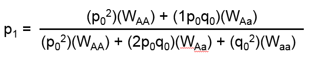
Note, it is not required that the fitness of a reference allele be set equal to 1. The three fitness coefficients need only to be proportional to each other.
The second system for modeling selection uses two user-specified coefficients, the selection coefficient, s, and dominance coefficient, h. The selection coefficient represents the degree of selection against the aa genotype group with respect to the AA genotype group. The dominance coefficient represents the degree to which selection also impacts the heterozygote. Selection and dominance coefficients can be expressed in terms of relative fitness coefficients as follows:
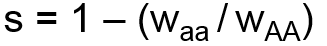 and
and
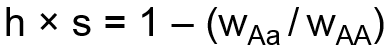
When selection and dominance coefficients are input by the user, the simulator will calculate the corresponding fitness coefficients, WAa and Waa, and set WAA equal to 1 as the reference. The above formula is then used to calculate the effect on allele frequency.
Both systems can be used to specify models of directional selection (also called positive selection), which in this context means that one allele is clearly favored and the other allele is clearly disfavored.
Models of over-dominance (also called heterozygote advantage), a form of balancing selection, can be specified using fitness coefficients. However, over-dominance cannot be specified in this simulator using selection and dominance coefficients. Other forms of balancing selection, such as frequency-dependent selection, are not implemented at this time.
Models of under-dominance (also called heterozygote disadvantage), a form of disruptive selection, can be specified using fitness coefficients. However, under-dominance cannot be specified using selection and dominance coefficients.
Two systems are available for defining selection models, but only one of these systems can be active at a time.
The first system requires user-specified relative fitness coefficients: WAA, WAa, and Waa, which represent the relative probabilities that an individual with a particular genotype reproduces. Typically one or more of the three fitness coefficients is set equal to 1 to serve as a reference, and the others are expressed as a fraction relative to the reference. After one generation of random mating, the allele frequency is modeled as:
Note, it is not required that the fitness of a reference allele be set equal to 1. The three fitness coefficients need only to be proportional to each other.
The second system for modeling selection uses two user-specified coefficients, the selection coefficient, s, and dominance coefficient, h. The selection coefficient represents the degree of selection against the aa genotype group with respect to the AA genotype group. The dominance coefficient represents the degree to which selection also impacts the heterozygote. Selection and dominance coefficients can be expressed in terms of relative fitness coefficients as follows:
and
When selection and dominance coefficients are input by the user, the simulator will calculate the corresponding fitness coefficients, WAa and Waa, and set WAA equal to 1 as the reference. The above formula is then used to calculate the effect on allele frequency.
Both systems can be used to specify models of directional selection (also called positive selection), which in this context means that one allele is clearly favored and the other allele is clearly disfavored.
Models of over-dominance (also called heterozygote advantage), a form of balancing selection, can be specified using fitness coefficients. However, over-dominance cannot be specified in this simulator using selection and dominance coefficients. Other forms of balancing selection, such as frequency-dependent selection, are not implemented at this time.
Models of under-dominance (also called heterozygote disadvantage), a form of disruptive selection, can be specified using fitness coefficients. However, under-dominance cannot be specified using selection and dominance coefficients.
-
Can X-linked/sex-linked selection be modeled? Can X-linked/sex-linked selection be modeled?
No. Currently selection occurring at a locus on an autosomal chromosome is implemented.
No. Currently selection occurring at a locus on an autosomal chromosome is implemented.
-
What is mutation? What is mutation?
Mutation is defined as a spontaneous change in genetic material. In some cases, mutation is a unique event. In other contexts, mutation can be conceptualized as a recurrent event, which occurs at some rate per generation. In the context of this simulator, mutation means that a given allele spontaneously changes into the other allele.
Mutation is defined as a spontaneous change in genetic material. In some cases, mutation is a unique event. In other contexts, mutation can be conceptualized as a recurrent event, which occurs at some rate per generation. In the context of this simulator, mutation means that a given allele spontaneously changes into the other allele.
-
How is mutation modeled in this simulator? How is mutation modeled in this simulator?
Mutation is modeled as a function of the forward (μ, A → a) and reverse (ν, a → A) mutation rates according the following formula:
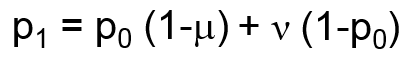
Mutation is modeled as a function of the forward (μ, A → a) and reverse (ν, a → A) mutation rates according the following formula:
-
What is genetic migration? What is genetic migration?
Genetic migration refers to the movement of outside alleles into the population of interest.
Genetic migration refers to the movement of outside alleles into the population of interest.
-
How is genetic migration modeled in this simulator? How is genetic migration modeled in this simulator?
Migration is modeled as a function of the migration rate, m, and the migrant allele frequency, pM, according to the following formula:
The migration rate corresponds to the proportion of alleles in the next generation that come from outside the population of interest. The migrant allele frequency is the allele frequency of the A allele in the set of alleles entering the population.
Note, this migration model may result in changes in allele frequency in the population of interest across generations. However, this model assumes there is no change in allele frequency in the migrant alleles. Therefore this model is applicable for many simplistic migration scenarios such as the “source-sink”, “continent-to-island”, “one island”, and “Wright’s island” models.
-
Can migration be modeled between two or more populations of interest? Can migration be modeled between two or more populations of interest?
No. The simulator assumes one population of interest (which may evolve across generations), and one static source of migrant alleles. Models where sources of migrant alleles are themselves changing in genetic composition are not currently implemented.
No. The simulator assumes one population of interest (which may evolve across generations), and one static source of migrant alleles. Models where sources of migrant alleles are themselves changing in genetic composition are not currently implemented.
-
What is inbreeding? What is the inbreeding coefficient? What is inbreeding? What is the inbreeding coefficient?
Inbreeding refers to the mating between two related individuals. Inbreeding in a population in excess of that expected due to chance alone can be described by the inbreeding coefficient, F.
Note, the inbreeding coefficient, F, is one of a family of “genetics F statistics”, also called fixation statistics, that measure various aspects of heterozygosity in individuals and strata within populations and between populations. In the context of this simulator, the inbreeding coefficient F is equivalent to Wright’s FIS and is equivalent to the average kinship coefficient between pairs of individuals in the previous generation.
-
How is inbreeding modeled in the simulator? How is inbreeding modeled in the simulator?
Inbreeding alone does not alter allele frequencies, and therefore it alone will not impact an allele frequency simulation. Inbreeding will alter the genotype proportions (and therefore impact the genotype frequency simulator). Other evolutionary forces such as selection operate on genotype groups, and therefore inbreeding may influence the actions of selection on a population.
Inbreeding is specified by the inbreeding coefficient, F, where genotype frequencies occur as follows:
P(AA) = p2 – Fpq
P(Aa) = 2pq + 2Fpq
P(aa) = q2 – Fpq
Inbreeding alone does not alter allele frequencies, and therefore it alone will not impact an allele frequency simulation. Inbreeding will alter the genotype proportions (and therefore impact the genotype frequency simulator). Other evolutionary forces such as selection operate on genotype groups, and therefore inbreeding may influence the actions of selection on a population.
Inbreeding is specified by the inbreeding coefficient, F, where genotype frequencies occur as follows:
P(AA) = p2 – Fpq
P(Aa) = 2pq + 2Fpq
P(aa) = q2 – Fpq -
What is assortative mating? What is assortative mating?
Assortative mating is the tendency of individuals to choose mates with similar (or dissimilar) genotypes. This bias influences the genotype frequencies of the next generation.
Assortative mating is the tendency of individuals to choose mates with similar (or dissimilar) genotypes. This bias influences the genotype frequencies of the next generation.
-
How is assortative mating modeled in the simulator? How is assortative mating modeled in the simulator?
Assortative mating alone does not alter allele frequencies, and therefore it alone will not impact an allele frequency simulation. Assortative mating will alter genotype proportions (and therefore will impact the genotype frequency simulator). Other evolutionary forces such as selection operate on genotype groups, and therefore assortative mating may influence the action of selection on a population.
Positive assortative mating is specified by the positive assortative mating fraction, α. The genotype frequencies in the next generation are:
P(AA) = [(1 – α)p2 + α(p2 + pq/2)] / D
P(Aa) = [(1 – α)2pq + α(pq)] / D
P(aa) = [(1 – α)q2 + α(q2 + pq/2)] / D
where D = [(1 – α)p2 + α(p2 + pq/2)] + [(1 – α)2pq + α(pq)] + [(1 – α)q2 + α(q2 + pq/2)]
-
Is negative assortative mating / disassortative mating modeled in the simulator? Is negative assortative mating / disassortative mating modeled in the simulator?
No, currently only simple-to-define scenarios of positive assortative mating are implemented.
No, currently only simple-to-define scenarios of positive assortative mating are implemented.
-
Can the simulator model multiple evolutionary forces simultaneously? Can the simulator model multiple evolutionary forces simultaneously?
Yes. One of the major strengths of simulation is that multiple forces can easily be applied simultaneously.
Yes. One of the major strengths of simulation is that multiple forces can easily be applied simultaneously.
Miscellany
-
Can the parameters of the simulation change across generations? Can the parameters of the simulation change across generations?
Generally, no. Once set, the parameters set by the user remain fixed for the duration of the simulation. However, some complex scenarios can be simulated in pieces, where the result (ending allele frequency) of a simulation be input as the starting point for a second phase under a new set of parameters. Multiple simulations can be strung together in this fashion to create multi-phase scenario.
Generally, no. Once set, the parameters set by the user remain fixed for the duration of the simulation. However, some complex scenarios can be simulated in pieces, where the result (ending allele frequency) of a simulation be input as the starting point for a second phase under a new set of parameters. Multiple simulations can be strung together in this fashion to create multi-phase scenario.
-
How can I cite the simulator? How can I cite the simulator? John R. Shaffer, Joshua Rogan. Online human population genetics simulator: a tool for genetics/genomics education and research. (2015) American Society of Human Genetics 65th Annual Meeting. Oct. 9, 2015. Baltimore, MD. Abstract #1701F.
John R. Shaffer, Joshua Rogan. Online human population genetics simulator: a tool for genetics/genomics education and research. (2015) American Society of Human Genetics 65th Annual Meeting. Oct. 9, 2015. Baltimore, MD. Abstract #1701F.
Simulator F.A.Q.
Simulator Usability
-
How can I create a graph of my simulation? How can I create a graph of my simulation?
To generate a new graph you can simply set the simulation parameters that you are interested in and click the "Generate Graph" button. You can then add more simulations to the existing graph by clicking the "Add Line" button. You can replace the existing graph with a new simulation by clicking the "Generate Graph" button."
To generate a new graph you can simply set the simulation parameters that you are interested in and click the "Generate Graph" button. You can then add more simulations to the existing graph by clicking the "Add Line" button. You can replace the existing graph with a new simulation by clicking the "Generate Graph" button."
-
How can I change the simulation parameters? How can I change the simulation parameters?
To change any of the simulation parameters you can open up the appropriate section by either clicking the checkbox to the left of the section name or the down arrow on the right. Once the section is opened you can either move the slider or click on the parameter value to directly input a new value using your keyboard.
To change any of the simulation parameters you can open up the appropriate section by either clicking the checkbox to the left of the section name or the down arrow on the right. Once the section is opened you can either move the slider or click on the parameter value to directly input a new value using your keyboard.
-
How can I activate a simulation parameter? How can I activate a simulation parameter?
The parameters automatically activate upon moving the slider or inputting a value. If the variable is active the corresponding slider will be shown in color and a check will be present next to the section name.
The parameters automatically activate upon moving the slider or inputting a value. If the variable is active the corresponding slider will be shown in color and a check will be present next to the section name.
-
How can I deactivate a simulation parameter? How can I deactivate a simulation parameter?
If a parameter is active (i.e., slider shown in color), you deactivate it by de-selecting the checkbox to the left of the section you would like to deactivate. Once a value is deselected the slider will be grayed out.
If a parameter is active (i.e., slider shown in color), you deactivate it by de-selecting the checkbox to the left of the section you would like to deactivate. Once a value is deselected the slider will be grayed out.
-
How can I zoom in the graph? How can I zoom in the graph?
To zoom in the graph simply click and drag across the area you would like to zoom in.
To zoom in the graph simply click and drag across the area you would like to zoom in.
-
How to pan left and right in the zoomed graph? How to pan left and right in the zoomed graph?
Click the directional button on the top right of the graph and click and drag to pan along the x axis of the graph.
Click the directional button on the top right of the graph and click and drag to pan along the x axis of the graph.
-
How can I reset the graph? How can I reset the graph?
To reset the graph click the circular arrow on the top right of the graph.
-
How can I save the graph as an image? How can I save the graph as an image?
To save the graph as an image file (jpg and png) click the triple dot in the upper left corner of the graph.

To save the graph as an image file (jpg and png) click the triple dot in the upper left corner of the graph.
-
How can I increase the contrast for printing or projecting? How can I increase the contrast for printing or projecting?
To choose a high contrast version of the graph for printing and projecting you can click the icon in the upper right hand corner of the variables section.
To choose a high contrast version of the graph for printing and projecting you can click the icon in the upper right hand corner of the variables section.
-
How can I view different legends? How can I view different legends?
Legends are automatically created for each simulation. Only the most recent simulation is shown. But, you can open legends of any previous simulation by clicking [Show Legend]
Legends are automatically created for each simulation. Only the most recent simulation is shown. But, you can open legends of any previous simulation by clicking [Show Legend]
-
Where can I find more information on the simulation parameters? Where can I find more information on the simulation parameters?
You can click the small question mark next to each variable in order to see a short explanation of the variable or click [Show Help] to open all of the parameter descriptions at once.
There is also a plethoral of help in the learn section of the this help area!
You can click the small question mark next to each variable in order to see a short explanation of the variable or click [Show Help] to open all of the parameter descriptions at once.
There is also a plethoral of help in the learn section of the this help area!
-
How can I generate a link (URL) for a simulation? How can I generate a link (URL) for a simulation?
You can generate a link (URL) for a set of simulation parameters by clicking on the . Navigating to this URL will prepopulate the set of simulation parameters that you currently have set. Feel free to modify the link to make the parameters more exact to your liking.
You can generate a link (URL) for a set of simulation parameters by clicking on the . Navigating to this URL will prepopulate the set of simulation parameters that you currently have set. Feel free to modify the link to make the parameters more exact to your liking.
-
How can I access the data represented in the graph? How can I access the data represented in the graph?
You can access the simulation data by clicking on the icon located in the top right corner of the Simulation Parameters section. This will take you to a seperate page containg scrollable, tab seperated x,y coordinates from each line that are currently on the graph. You can easily copy and paste this into your favorite data manipulation program to perform additional analysis.
You can access the simulation data by clicking on the icon located in the top right corner of the Simulation Parameters section. This will take you to a seperate page containg scrollable, tab seperated x,y coordinates from each line that are currently on the graph. You can easily copy and paste this into your favorite data manipulation program to perform additional analysis.
Technical Questions
-
How can I submit a bug or potential new feature? How can I submit a bug or potential new feature?
You can navigate to the Report a Problem page to either submit a bug/error or suggest new features.
You can navigate to the Report a Problem page to either submit a bug/error or suggest new features.
-
How was this application created? How was this application created?
This application was created by Josh Rogan and commissioned by Dr. John Shaffer, Assistant Professor of Human Genetics at the University of Pittsburgh.
This application was created by Josh Rogan and commissioned by Dr. John Shaffer, Assistant Professor of Human Genetics at the University of Pittsburgh.
-
How was this application developed? How was this application developed?
The graphing application is powered by JavaScript with heavy usage of Web Workers for performance. The graphing library for both the simulators is CanvasJS as it out performed all other responsive graphing libraries. The frontend design is built with the responsive frontend framework Twitter Bootstrap. The backend utilizes the PHP framework Laravel heavily utilizing the Blade templating engine.
Everything Else:The graphing application is powered by JavaScript with heavy usage of Web Workers for performance. The graphing library for both the simulators is CanvasJS as it out performed all other responsive graphing libraries. The frontend design is built with the responsive frontend framework Twitter Bootstrap. The backend utilizes the PHP framework Laravel heavily utilizing the Blade templating engine.
Everything Else: -
How can I support this project? How can I support this project?
To support this project you can submit bugs, submit issues to the github repository, or contact us!
To support this project you can submit bugs, submit issues to the github repository, or contact us!